


Abstract
Ride sharing—the bundling of simultaneous trips of several people in one vehicle—may help to reduce the carbon footprint of human mobility. However, the complex collective dynamics pose a challenge when predicting the efficiency and sustainability of ride sharing systems. Standard door-to-door ride sharing services trade reduced route length for increased user travel times and come with the burden of many stops and detours to pick up individual users. Requiring some users to walk to nearby shared stops reduces detours, but could become inefficient if spatio-temporal demand patterns do not well fit the stop locations. Here, we present a simple model of dynamic stop pooling with flexible stop positions. We analyze the performance of ride sharing services with and without stop pooling by numerically and analytically evaluating the steady state dynamics of the vehicles and requests of the ride sharing service. Dynamic stop pooling does a priori not save route length, but occupancy. Intriguingly, it also reduces the travel time, although users walk parts of their trip. Together, these insights explain how dynamic stop pooling may break the trade-off between route lengths and travel time in door-to-door ride sharing, thus enabling higher sustainability and service quality.
Export citation and abstract BibTeX RIS

Original content from this work may be used under the terms of the Creative Commons Attribution 4.0 licence. Any further distribution of this work must maintain attribution to the author(s) and the title of the work, journal citation and DOI.
1. Introduction
Emergent collective dynamics make it difficult to understand and predict the behavior of complex systems. [1–9]. For instance in mobility systems, many different agents with various aims interact, which makes it hard to quantify key indicators like the efficiency. Methods from statistical physics, like network theory [10], scaling analysis [11, 12], or mean-field theory [13] can help to overcome this challenge.
In human mobility in particular, understanding the efficiency of different services is crucial to enable a shift towards more sustainable mobility. Individual motorized mobility is highly inefficient with only about 1.3 passengers per car on average [14]. Making human mobility more sustainable requires a reduction of total route length driven and simultaneously fewer numbers of vehicles. Arguably, the most influential factor toward achieving this goal is a substantial increase of the average number of passengers per vehicle.
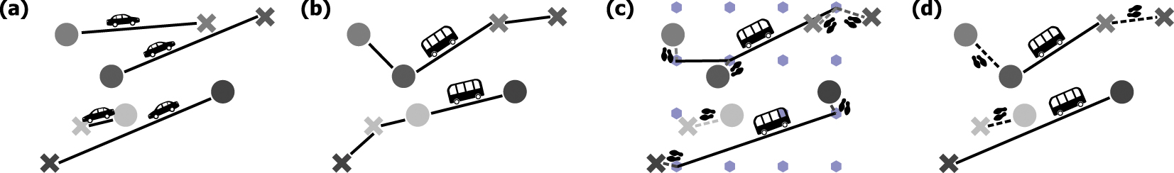
Ride sharing (also called ride pooling) [10, 12, 15–17] constitutes a promising tool to bundle multiple user trips in a single vehicle—for instance micro- or minibuses with typically 4 to 24 seats [18]. While each individual user incurs a small detour on their trip, the ride sharing buses serve the users with a significantly shorter route length than in individual mobility where each user drives in their own car [16] (figures 1(a) and (b)).

Figure 1. Route length and travel time depend on mode of transport. (a) Individual mobility is the fastest mode of transport but requires longest total route length. (b) Standard ride sharing serves users from door to door. Ride sharing reduces total route length by combining trips and requires fewer (but larger) buses. Users may become slower due to detours and between stops. (c) Static stop pooling with fixed stop positions (purple hexagons) reduces the number of stops but requires users to always walk part of their trip which might increase travel time even further. (d) Dynamic stop pooling with flexible stop positions combines efficient public transportation and adaptive ride sharing and might thus save both total route length and user travel time despite users might walk a part of their trip.
Download figure:
Standard image High-resolution imageHowever, many small detours to pickup users individually in door-to-door ride sharing services increase both the total route length (reduced sustainability) as well as user travel times (reduced service quality). Stop pooling offers the possibility to reduce these detours: if users walk a short distance to nearby stops (as in public transportation), the buses stop less often and save some door-to-door detours [19–24].
Fixed positions of stops as in line bus services enable a simple implementation of stop pooling. Each user walks to and from the closest stop, reducing the number of possible combinations of trips and thus the computational effort of the algorithm that bundles the trips. Such a static implementation of stop pooling with fixed, prescribed stops (figure 1(c)) reduces the relative route length but typically increases the user travel time [19–22]. To overcome this challenge, we here propose dynamic stop pooling, where both bus route and user stops are adapted to current demand (figure 1(d)). Two recent algorithmic models on dynamic stop pooling [23, 24] suggest the possibility for both shorter total route length and simultaneously shorter travel time but do not analyze the mechanisms underlying this observation.
Most studies of ride sharing services focus on operational aspects, including user behavior and economics [16, 25–27] or algorithmic optimization [15, 28, 29], especially in contrast to individual mobility. Recent studies have begun to develop an understanding of the collective dynamics of ride sharing fleets from a complex systems perspective, revealing how these dynamics impact the efficiency of ride sharing across settings [10–13]. However, an analysis of the collective dynamics induced by dynamic stop pooling and their effect on the ride sharing service quality is still missing.
In this article we present, first, a simple multi-agent model for ride sharing that captures the trade-off between route length and travel time in door-to-door ride sharing; second, include dynamic stop pooling and show how it may decrease the travel time by reducing detours between stops, and third, demonstrate how this enables dynamic stop pooling to break the ride sharing trade-off. We conclude that dynamic stop pooling may improve both route length and travel time simultaneously by adjusting the maximal walk distance of the users and the number of buses. Dynamic stop pooling could thus allow to establish a fast, flexible and sustainable ride sharing service.
2. Model
2.1. Ride sharing
The collective dynamics of ride sharing is determined by the interaction of user requests and the buses serving them. Let us consider the following simple model for ride sharing: users request a service to transport them from their origin to their destination as soon as possible; the service provider operates a fleet of  buses to serve these users; when a request is posed, it is assigned to a bus according to an assignment algorithm (see section 2.3). That is, origin and destination are inserted at appropriate positions into the current route of the bus as pickup and drop-off stops. In the model the order of the scheduled stops once assigned does not swap, even if later requests are inserted into the bus route. Over time, the buses drive with velocity
  and visit all scheduled stops one after each other (figure 2, left panel).

Figure 2. Dynamic stop pooling avoids door-to-door detours by combining close-by stops. In door-to-door ride sharing (Left), the bus drives to each stop resulting in an overall route with many small detours (black line). Dynamic stop pooling may avoid these detours by combining close-by stops, yet keeps the overall route structure similar (compare red line). In detail, some users walk to a nearby stop closer than pool radius r (Right). Their stops are served indirectly. If origin and destination are closer than 2r, users walk completely and do effectively not use the service. Their stops are rejected. Ultimately, the bus serves only the remaining stops directly.
Download figure:
Standard image High-resolution image2.2. Dynamic stop pooling
With dynamic stop pooling, users may have to walk a short distance at their origin and destination—at most pool radius
 per stop. Users walk from their origin to a close stop, which has to be already planned, if they reach it before the bus; similarly, they walk from a close stop to their destination. Thus, the buses can serve multiple users at one stop and save stops and related door-to-door detours.
Stops are either served directly or indirectly, or rejected (not served). If served directly, the user is picked up or dropped off directly at their desired stop; if served indirectly, the user walks to or from a close directly served stop. To avoid users to walk further than their requested trip length and to waste time (both their own and that of the service fleet), people with requested trip length  are rejected and walk completely. In contrast to directly and indirectly served stops, their stops are not served by the buses.
Figure 2 illustrates the difference between dynamic stop pooling and door-to-door ride sharing as well as the resulting stop types. These stop types yield three distinct user types: if both origin and destination are served directly, users do not walk; if one or two stops are served indirectly, users walk partially; otherwise the request is rejected and users walk completely.
2.3. Setting
We model the dynamics of the ride sharing service by Monte Carlo simulations [30]. The requests follow a Poisson process [31] with mean field request rate  where the position of the origin is distributed uniformly in a unit square with periodic boundaries. Destinations are distributed uniformly in a disk around the origin with maximal trip length
  such that diagonal trips are not more probable than others. The trip length (tl) of all users is thus distributed according to

with an average trip length  (see supplementary material A, equation (S2)) (https://stacks.iop.org/
NJP/24/023034/mmedia).
(see supplementary material A, equation (S2)) (https://stacks.iop.org/
NJP/24/023034/mmedia).
We introduce stop pooling with the same pool radius for all users, independent of their trip length. To avoid that users walk further than their trip length, we reject users with  , where the factor 2 captures the fact that users may walk a distance r from their origin as well as to their destination. We rescale the pool radius as

to better reflect the effect on the users. For minimal relative pool radius
 (
( ), users do not walk (door-to-door ride sharing). For
  , the relative pool radius
  gives the percentage of the maximal trip length that users are required to walk. For maximal relative pool radius
  (
( ) all users walk completely and no ride sharing takes place anymore.
As the pool radius increases, more users are not served and walk completely. The ratio  of rejected stops, which is similar to the ratio of rejected users, follows directly from the fraction of trips with lengths
  by integrating the trip length distribution
  only for rejected users, i.e. from 0 to 2r, as

It only depends on the relative pool radius  .
.
When a request arrives, we assign it to one of B buses and insert pickup and drop off stops (unless the user walks to other stops) into the current route of the bus. We determine the assignment and routing according to a simple algorithm that exclusively minimizes the bus route length, i.e. the sum of the distances of all subsequent stops in its route. When a request appears, the algorithm calculates for each bus how to insert the origin and destination with minimal additional route length. For this purpose, it iterates over all currently planned stops in the bus route to check whether the user could be served indirectly via this planned stop (if  ) or, if not, how much an insertion of the new stop would increase the route length. In the end, the algorithm assigns the request to the bus with shortest route length after inserting the request. If origin and destination are far from planned stops, the bus would pick up and deliver the user directly from and to their requested location. If there are planned stops near the origin or destination, the algorithm favors stop pooling to minimize the route length.
The buses drive with velocity vb on the shortest path from stop to stop, serving all assigned users. Users walk to and from their pooled stops or their whole trip on the shortest path with velocity  . For simplicity, we consider buses with infinite capacity
  and zero time to decelerate, park, serve users and accelerate again at each stop (zero stopping time). This setting marks a lower bound for the efficiency of stop pooling because it can only save route length but no stopping time.
For all simulations illustrated in the figures, we take a constant request rate  and bus velocity
  and vary the number of buses
 ![$B\in [30,35,\dots ,60]$](https://content.cld.iop.org/journals/1367-2630/24/2/023034/revision3/njpac47c9ieqn26.gif) and the relative pool radius
and the relative pool radius  to analyze the influence of dynamic stop pooling on door-to-door ride sharing, modeled by
  . All other parameters are kept constant. In particular, we use exactly identical requests (request times, origins and destinations) in the different simulations, not only similar request distribution. In this way, we show how stop pooling can help to improve a certain service with given demand—e.g. in a given city.
Clearly, stop pooling can only take place with stops of other users. Thus, users first have to share rides, before they can pool stops. The service is in the ride sharing regime, i.e. it has to bundle user trips, if more trip length is requested than the buses can travel per time. The load

defined by Molkenthin et al [12] characterizes the ride sharing regime by  . Here,
  is the average trip length requested per time and
  the maximal distance all buses can travel together per time. The load is a lower bound for the average occupancy of the buses [12]. As long as
  , the buses are on average always occupied by at least one user and are almost never idle.
The higher the load x, the more user trips need to be bundled to serve all requests. However, high loads come along with high computation cost (of the assignment algorithm), high occupancy, and high user travel time and are unfeasible and unrealistic. To be well in the ride sharing regime without too high loads, we choose initial loads (door-to-door ride sharing) ![${x}_{0}\in [3,6]$](https://content.cld.iop.org/journals/1367-2630/24/2/023034/revision3/njpac47c9ieqn33.gif) (compare parameters above). That means, three to six times more route length is requested than the buses can serve. In consequence, on average at least three to six users are in a bus per time step who can pool their stops. Due to detours and longer travel times, the actual occupancy is typically much larger, especially in settings with only few buses.
(compare parameters above). That means, three to six times more route length is requested than the buses can serve. In consequence, on average at least three to six users are in a bus per time step who can pool their stops. Due to detours and longer travel times, the actual occupancy is typically much larger, especially in settings with only few buses.
2.4. Observables
We start our simulations with B empty buses randomly distributed in the unit square and wait for some time  until the bus occupancy and the length of the planned routes have equilibrated. We measure our observables in a fixed observation window
 ![$\Delta T=100, t\in [100,200]$](https://content.cld.iop.org/journals/1367-2630/24/2/023034/revision3/njpac47c9ieqn35.gif) , in the steady state after equilibration. In this window, approximately
, in the steady state after equilibration. In this window, approximately  users are served. We consider only request with delivery in the observation window. Because we simulate for such a long time and so many users, we observe well defined average values. The standard error of the mean for our observables is very small and thus negligible in the figures presented below.
2.4.1. Route length
The total route length  is the sum of all bus route lengths. The route length
  of bus
  is the sum over all stop distances of the route of the bus. We normalize
  by the ideal total route length in individual mobility
  , the sum of all
  user trip lengths
  . The rescaled observable relative route length

quantifies how much longer/shorter the buses drive to serve the users compared to each user going by car individually. Here,  is the average probability for the buses to become idle. For
  , the buses would in total drive further than cars in individual mobility. For
  , the service requires less bus route length to serve all users than individual mobility and is
  times more efficient in route length. For
  , no buses drive at all, the service does not serve anyone. This only occurs for
  when all users walk completely.
Over a constant observation time T, the total route length by the bus fleet is directly proportional to the idle time of the buses. In particular, if buses are never idle due to sufficiently high load,  for
for  , the total route length
  does not change with the relative pool radius
  or the load
  . Similarly, the total sum of the user trip distance
  depends on the request rate
  and the trip length distribution but not on
  such that the relative route length is independent of
  in the ride sharing regime.
We take energy required and emissions caused to be proportional to the total route length driven, neglecting the influence of vehicle size or capacity compared to private vehicles. The relative route length  thus quantifies the energy consumption and emissions of a ride sharing system compared to ideal individual mobility. For
  , we thus consider the system to be ecologically more sustainable.
2.4.2. Travel time
Usually, users pay for the reduced relative route length with longer travel times than in individual mobility. We measure the average of all  user's travel time, which is the time between request and arrival at the destination. We normalize this average travel time by the ideal average travel time in individual mobility when all users are served immediately, without detour and with bus velocity
  . This relative travel time
 reads
reads

The relative travel time measures how much slower users are compared to the ideal travel time. Because we measure a user related observable, we include all users into the relative travel time. Rejected users simply contribute their walk time  . The minimal possible relative travel time in ideal individual mobility equals one. For
  , users are
  times slower than in individual mobility. In the example study below we have
  that measures the relative travel time when all users walk completely.
3. Results
3.1. Door-to-door ride sharing
First, we analyze how door-to-door ride sharing without stop pooling,  , with fixed request rate scales for different fleet sizes
  . Relative travel time and relative route length scale oppositely: the relative route length increases with increasing number
  of buses (figure 3(a)); the relative travel time decreases with increasing
  (figure 3(b)). Joining these findings for similar
  shows that ride sharing services pay with increased relative travel time when reducing the relative route length by varying and vice versa (figure 3(c)). We thus identify a trade-off between relative route length and relative travel time for door-to-door ride sharing. For given requests we cannot improve both at the same time (in analogy to [32]).

Figure 3. Trade-off between relative route length and relative travel time in door-to-door ride sharing. (a) The relative route length  increases approximately linearly with increasing number
  of buses because
 ![$x\in [3,6]$](https://content.cld.iop.org/journals/1367-2630/24/2/023034/revision3/njpac47c9ieqn75.gif) for constant
for constant  are sufficiently high that buses are almost never idle (
 , compare equation (5)). (b) At the same time, the relative travel time
  decreases. The fewer buses, the more route can be saved but the longer do users travel. (c) Relative travel time (from panel (b)) vs route length (from panel (a)) joined by similar B encoded by small numbers beneath the curve. If reducing the relative travel time, the relative route length increases in return and vise versa. It is hence impossible to improve both at the same time by just varying the number
  of buses in door-to-door ride sharing. Black dashed lines are guides to the eye.
Download figure:
Standard image High-resolution image3.2. Ride sharing with dynamic stop pooling
With dynamic stop pooling, users may walk to and from a close stop. For  , users do not walk (door-to-door ride sharing); for
  , all users walk completely. Below, we explore the influence of any
 ![$\tilde{r}\in [0,1]$](https://content.cld.iop.org/journals/1367-2630/24/2/023034/revision3/njpac47c9ieqn82.gif) on ride sharing in the model.
on ride sharing in the model.
3.2.1. Fewer stops
The number of stops reduces in two ways: if users are served indirectly and walk to a nearby stop or if users are rejected and walk completely. The second form of stop reduction is clearly undesirable for the users. Thus, the ratio of rejected users, which is the same as the ratio  of rejected stops relative to the total number of stops, should be rather small,
  .
.
The ratio  of rejected stops is proportional to the fraction of requests with destination in a circle with radius
  around the origin, because these users are rejected and walk completely. With a uniform request distribution (see section 2),
  grows quadratically in
  and is exactly equal to
  in terms of the normalized pool radius (see section 2, equation (3)). The ratio
  of served stops, which consists of the ratio
  of directly served stops and the ratio
  of indirectly served stops, thus decreases quadratically with
  as
as

For minimal relative pool radius  (door-to-door ride sharing), the buses serve all stops directly:
  . For maximal pool radius
  , the buses serve no stops
  and all users walk completely, ωr = 1. Consequently, only small relative pool radii
  are feasible so that most users are served.
Simulations show that the ratio  of directly served stops reduces with increasing relative pool radius faster than the ratio
  of served stops (figure 4(a)). The remaining fraction
  of stops is served indirectly. This ratio
  of indirectly served stops quantifies the degree of actual stop pooling: how many stops are combined with others (instead of how many stops are rejected). For small pool radii, it increases and then decreases again with the relative pool radius when complete walking dominates (figure 4(b)). First, more and more users walk to close stops with increasing relative pool radius. When the relative pool radius increases further, more and more of these users are rejected and walk their whole trip. Rejected stops replace indirectly served ones.

Figure 4. Relative route length stays roughly constant although dynamic stop pooling saves stops. (a) The ratio  of directly served stops decreases monotonically with
  , faster than the served stop ratio
  (blue line, see equation (7)), which divides the saved stops into rejected
  (shaded grey) and indirectly served stop ratio
  (shaded orange). (b) The indirectly served stop ratio
  first increases and then decreases again with increasing
  . Moreover,
  increases with decreasing
  (and constant
  ) for
) for  . That is, the more users share one bus, the more stops can be pooled. In general, stop pooling is only feasible for small pool radii
  where most users are served (ωs, blue line) and the minority of users is rejected (ωr, shaded grey). (c) Rejections reduce the load
 . For sufficiently small
  , the load (black dashed lines according to equation (8)) is high,
  , and the system is in the ride sharing regime, such that all buses are busy at all times. For very high
  , the load decreases to
  and almost no rides are served anymore. Buses have to wait for incoming requests. (d) Roughly constant relative route length
  for small
  due to busy buses for
  (cp equation (5)). Only for sufficiently large
  , the load falls below 1 (see panel (c)) and the route length decreases to zero when all users walk completely for
  .
.
Download figure:
Standard image High-resolution imageThe potential of stop pooling increases with fewer buses. Since more users share a bus, the bus visits more stops that are on average closer together and can be pooled easier. Overall the more users share a bus, the higher is the potential of dynamic stop pooling.
3.2.2. Constant route length
The load  measures how much trip length is requested compared to how far the buses can drive in total per time step (see section 2, equation (4)). It is a lower bound for the average occupancy
  of the buses [12]—the average number of users per bus at any point in time. Because rejected users do not contribute to the load
  , it depends on the relative pool radius as (derivation in supplementary material A)

where  denotes the load for door-to-door ride sharing with
  . The load decreases with increasing relative pool radius (see figure 4(c)). Due to the high initial values
 ![${x}_{0}\in [3,6]$](https://content.cld.iop.org/journals/1367-2630/24/2/023034/revision3/njpac47c9ieqn130.gif) , the load stays larger than one for most feasible pool radii. Consequently, the buses are typically occupied and thus remain busy almost all the time (
, the load stays larger than one for most feasible pool radii. Consequently, the buses are typically occupied and thus remain busy almost all the time ( , compare equation (5)). Because they move with constant velocity, the buses drive the same route length in this time (observation window). Since the requests and their ideal total route length also stay the same, we measure a constant relative route length (figure 4(d)). Only for (infeasibly) high relative pool radii close to one, the load falls below one. Buses become idle from time to time and wait for new requests without driving. The relative route length decreases until buses do not drive at all when all users walk at
  .
.
3.2.3. Faster users
A constant relative route length despite saved stops might initially seem counter-intuitive. But the route length stays only constant from the point of view of the buses. Users see less of this route length, since they are faster and spend less time waiting for and driving in the buses (figures 5(a) and (b)). The relative travel time becomes minimal for some intermediate pool radius  where neither all users are served from door to door (
 ) nor everyone walks (
 ).
).

Figure 5. Dynamic stop pooling reduces relative travel time and occupancy for sufficiently small  . (a) The relative travel time is minimal for some intermediate relative pool radius (
 ). This minimal relative travel time is lower than the relative travel time for door-to-door ride sharing (
 ) and lower than the relative travel time
  (dashed line) when all users walk completely (
 ). In general, the relative travel time decreases with
  (as shown in figure 3). (b) The relative travel time splits into drive, wait and walk time, shown here for
  (cp panel (a)). The wait and drive time decrease for increasing
  . This effect is only partially explained by rejected users who walk completely and do not drive/wait. Additionally, buses avoid door-to-door detours, further reducing the drive and wait time of the remaining users. Reduced drive and wait time overcompensate the increasing walk time for small enough
  such that the overall relative travel time decreases. For large
  , the walk time dominates and the relative travel time increases up to
  . (c) The average occupancy
  decreases with increasing
  and
and  . Dynamic stop pooling thus allows to use smaller buses than door-to-door ride sharing.
Download figure:
Standard image High-resolution imageDynamic stop pooling can reduce the relative travel time by making few users walk partially or completely and in turn reducing the drive and wait time. This reduction on average overcompensates the additional walk time for sufficiently small  (figure 5(b)). This comparison not only holds for the averages, but extends to the full travel time distributions as well (cp supplementary material B 2).
3.2.4. Lower bus occupancy
Since users spend less time in the buses (see figures 5(a) and (b)), the average occupancy  of the buses reduces with dynamic stop pooling (figure 5(c)). Fewer buses may serve the same requests with the same average occupancy that would have been impractically high for door-to-door ride sharing. For example 45 buses require on average
  seats with
  = 0, but only
  with intermediate relative pool radius
  , which could be served by a minibus.
The magnitude of this effect increases the more users initially share a bus and goes beyond the pure rejections due to users walking completely (see supplementary material C). When fewer buses serve the same requests, more users share the same bus such that dynamic stop pooling saves more stops, relative travel time and occupancy (figures 4(a) and 5(a) and (c)).
In summary, with increasing (small enough) relative pool radius while keeping all other parameters constant (I) buses drive the same total route length because they are still busy all the time, (II) buses stop less often because more stops are pooled, thus (III) reducing the waiting time and detour for users and ultimately (IV) resulting in smaller average travel times for users despite walking further.
3.3. Dynamic stop pooling breaks trade-off
With fixed relative pool radius  , lowering
  reduces the relative route length (figure 4(d)) but increases the relative travel time (figure 5(a)). The door-to-door ride sharing trade-off between relative route length and relative travel time when only varying
  persists with dynamic stop pooling for constant
  (figure 6). Raising the relative pool radius
  with fixed
  decreases the relative travel time but keeps the relative route length roughly constant (as long as
  is feasibly small). However, in combination, it is possible to decrease the relative route length while keeping the relative travel time constant by reducing
  and raising
  simultaneously. We no longer pay automatically with higher relative travel times for shorter relative route lengths. Dynamic stop pooling breaks the ride sharing trade-off between route length and travel time.

Figure 6. Stop pooling breaks the ride sharing trade-off between relative route length and relative travel time. With fixed relative pool radius  (shades of blue), the service shows the same trade-off between the relative travel time and the relative route length when varying
  (denoted by the small numbers beneath the data points), e.g. for (i) → (ii) (cp figure 3). However, the increase in the relative travel time is lower for higher relative pool radii. Increasing
  shifts the service to a lower relative travel time for sufficiently small
  (cp figure 5). Together, increasing both
  and reducing
  results in decreased relative route length while keeping the relative travel time approximately constant, (i) → (iii). Stop pooling thus breaks the ride sharing trade-off. Detailed data on the scenarios (i), (ii) and (iii) is given in the table on the right. Scenarios (i) and (ii) yield bad relative route length or relative travel time (red background), respectively. Scenario (iii) with dynamic stop pooling yields better results for both (green background).
Download figure:
Standard image High-resolution image
This breaking of the trade-off is a qualitative novelty of dynamic stop pooling as opposed to static stop pooling or door-to-door ride sharing. Existing studies of static stop pooling (that focus on reduced route length and increases shareability) observed longer travel times [19–21]. So far, only studies with dynamic stop pooling (including this article) have observed reduced travel times [23, 24].
Instead of trading short bus route lengths for high user travel times, it is sufficient to let users walk a short part of their trips if both bus route and stop positions are flexible.
To better understand this effect, consider the three scenarios illustrated in figure 6. In scenario (i), a door-to-door ride sharing service delivers the users with 45 buses. If the service provider decides to only use 40 buses (scenario (ii)), the route length reduces by 11%, but users travel on average 23% longer due to the ride sharing trade-off. The provider risks losing users. In scenario (iii), 40 buses with dynamic stop pooling serve the users at the same speed as in scenario (i), if the users walk up to 10% of their maximal trip length. Both relative route length and relative travel time are smaller than in scenarios (i) and (ii) (figure 6). The provider saves 11% route length, and 11% of the buses without increasing the relative average travel time or requiring much larger buses. The same holds for the distributions of the user travel times (see supplementary material B 2).
In return, only one percent of the users walk completely. Around half of the users do not walk at all, and the remaining partially walking users walk on average 8% of their trip. Averaged over all users, they walk only 5% of their trip, thereby enabling a more sustainable ride sharing service with slightly faster users.
4. Discussion
The simple model introduced above captures fundamental spatio-temporal interaction of various agents of ride sharing systems with dynamic stop pooling. We systematically analyzed the collective system dynamics for varying pool radius  and number
  of buses. Other parameters like the average bus velocity, the request rate and the average requested trip length are summarized in a system-wide load
  (equation (8)), cf also [12]. The results demonstrate that dynamic stop pooling may break the trade-off that is prevalent in door-to-door ride sharing systems between reducing relative bus route length and reducing relative user travel time (figure 6 and section 3.1).
Dynamic stop pooling increases ride sharing efficiency by reducing the number of directly served stops (section 3.2.1). It thereby avoids many small door-to-door detours and decreases the occupancy of the buses if some users walk a short distance to a dynamically determined stop, in contrast to static stop pooling where every user would have to walk to a prescribed stop. Dynamic stop pooling thereby decreases the relative travel time (section 3.2.3) while keeping the relative route length constant (section 3.2.2)—a novel quality for ride sharing systems (section 3.3). As a consequence, upon increasing the maximum walk distance of dynamic stop pooling, a smaller number of buses may serve the same number of requests without longer travel times and without needing larger buses (section 3.3). Dynamic stop pooling may thus help to make ride sharing ecologically more sustainable by reducing the number of buses, resulting in lower energy consumption and emissions, without negatively impacting flexibility, service quality and travel times.
The general mechanism of breaking the ride sharing trade-off relies on the interplay of two general conditions: first, dynamic stop pooling is only possible in the ride sharing regime,  , where buses do not serve all users one after another, because (in a given time) the sum of the trip length of all users is larger than the distance that the buses are able to drive. Thus, multiple users share a bus, which allows to pool their stops. Since stops close to each other (in space and time) may be pooled, dynamic stop pooling becomes more efficient for higher loads
  (i.e. for fewer buses or higher request rate) with many stops per bus, whereas the influence of dynamic stop pooling vanishes for small loads x with few stops per bus.
Second, to neutralize the increase in the travel time with reducing  (negative effect of the trade-off) the travel time needs to decrease enough with
  . The travel time only decreases for small enough
  and up to some minimal value for each
  . If reducing
  too much, even the maximal decrease of the travel time for optimal
  might not neutralize the increase in the travel time due to reduction of
  completely. For instance when reducing
  in the above example from 60 to 30, which would half the relative route length, however much increasing
  will yield a higher travel time (all
  with
with  are higher than
  with
with  and
and  , cp figure 5). Dynamic stop pooling is unable to completely neutralize this high decrease in
  and only buffers it. But for small reduction in
  , we can observe a shorter route length (due to
  reduction) without longer travel time when increasing
  . The same effect could be observed if a shorter route length compensates an increasing travel time (cp [23, 24]). This condition is typically fulfilled for small pool radii where the service avoids small door-to-door detours without rejecting a large fraction of users due to additional benefits to the remaining users (see supplementary material C). High pool radii are not feasible since most users walk, increasing their travel time, and almost no served stops remain to be pooled.
These arguments hold under more general conditions than those studied in our simplified model. First of all, different assignment algorithms and different delay or capacity constraints may reduce the options to pool stops. Similarly, walking may not be possible for all users. While these aspects may limit the overall potential of dynamic stop pooling, it does not affect the qualitative mechanisms described above. Moreover, additional aspects including substantial stopping times, deceleration and acceleration, and the influence of traffic density on lane-switching, overall vehicle velocity and stopping times may even increase the benefits of stop pooling in terms of added comfort and security. (For a more detailed discussion of the robustness, see supplementary material D.)
Our simple model setting may represent real world urban centers with high request densities at highly frequented locations although the continuous space strongly reduces the overlap of requested trips resulting in high relative travel times (see supplementary material section B 1). Equating the length and time scales in our model to typical conditions in Manhattan with a total area of 59 km2 (8 km per length unit) and average velocity 10 km h−1 [33], the simulated request rate corresponds to 11.25 requests per minute or less than 5% of the typical taxi request rate in Manhattan (approximately 400 000 daily [10]). Already for such a small fraction of requests and number of buses—chosen for the sake of computational feasibility—dynamic stop pooling may break the ride sharing trade-off. Furthermore, our results remain robust for larger request rates and numbers of buses. Indeed, sharing rides and pooling stops becomes even easier resulting in shorter relative travel times for comparable loads and similar relative savings from stop pooling (see supplementary material D for supporting simulations). Moreover, we find the same qualitative result even if rejected users drive individually instead of walk (see also supplementary material D).
Overall, we have identified the joint dynamic interaction of walking, routing buses, and dynamically pooling stops as the core mechanism to break the ride sharing trade-off. Better understanding the influence of dynamic stop pooling and the underlying mechanisms may thus help to enable simultaneously more sustainable and more flexible shared mobility.
Acknowledgments
The authors thank Verena Krall, Felix Jung and all members of Chair for Network Dynamics for valuable discussions. This work was partially supported by the Volkswagen Foundation under Grant No. 99720. CL acknowledges support from the German Federal Environmental Foundation (Deutsche Bundesstiftung Umwelt). The authors are grateful to the Centre for Information Services and High Performance Computing (ZIH) TU Dresden for providing facilities for high throughput calculations.
Conflict of Interest
The authors declare no conflicts of interest.
Data availability statement
The data that support the findings of this study are available upon reasonable request from the authors.